Network business models should take account of geographical realities such as varying
customer densities and backhaul costs, but typically data is only available at an
aggregate level in the early stages of business planning. This refresher article
illustrates how STEM can make a realistic allowance for slack equipment capacity
across a distributed network, how it can perform a site-by-site calculation when
the data becomes available without your head exploding, and how the overall results
typically compare.
Matching installed equipment capacity to total subscriber demand
 To
illustrate this article, we are going to look at the business model for a new ISP
which aims to deploy its own DSLAMs across multiple exchange sites under one of
the now common local-loop unbundling (LLU) regimes. Although the full business model
would consider a detailed service portfolio in order to forecast the aggregation
of voice and data traffic, we are just going to focus on the number of required
ports on a DSLAM at any given site.
To
illustrate this article, we are going to look at the business model for a new ISP
which aims to deploy its own DSLAMs across multiple exchange sites under one of
the now common local-loop unbundling (LLU) regimes. Although the full business model
would consider a detailed service portfolio in order to forecast the aggregation
of voice and data traffic, we are just going to focus on the number of required
ports on a DSLAM at any given site.
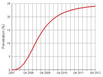 The
business model will run for five years from 2008–12, and STEM will generate the
results in quarters throughout. For the prototype site, we assume an addressable
market of 5000 households, and model penetration as an S-curve increasing towards
a saturation of 25% market share, i.e. around 1250 subscribers by Q4 2012.
The
business model will run for five years from 2008–12, and STEM will generate the
results in quarters throughout. For the prototype site, we assume an addressable
market of 5000 households, and model penetration as an S-curve increasing towards
a saturation of 25% market share, i.e. around 1250 subscribers by Q4 2012.
We assume that the new operator will buy and deploy equipment capacity in units
of full shelves of 480 ports (= 20 cards per shelf × 24 ports per card), and that
a single DSLAM can accommodate up to four shelves = 1920 ports.
This results in an initial deployment of one shelf for service launch in Q1 2008,
and then the second and third shelves being added as the demand increases. How quickly
this happens depends on the overall subscriber growth rate. STEM matches the installed
equipment capacity to the total demand from subscribers automatically. Notice the
blue line on the chart below showing the slack capacity, which varies in the range
0–497 ports, peaking immediately after the installation of a new shelf.
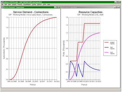
Service demand and installed equipment capacity
Usually we would use a maximum utilisation constraint to cause the second shelf
to be installed before 100% utilisation of the first shelf is achieved, matching
what the operator’s technical staff would do in practice. However, this is equivalent
to working with a smaller unit capacity, and the issue is disregarded in this model
to keep things simple.
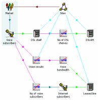
Allowing for slack equipment capacity across a distributed network
Of course, modelling demand at just one site is not very challenging: the complexity
arises from varying characteristics across multiple sites, and the interconnections
between them. Now we will extend the model to consider nine sites as a clear illustration
of principles which could be applied equally well to 90 sites. In fact the point
of this article is to show how you can readily calculate perfectly ‘good enough’
results for an unlimited number of sites without having to model them individually.
STEM’s built-in deployment feature allows you to express the fact that a single
demand is spread over one or more physically separate sites: in this case, local
exchange sites in different towns.
The initial model was already structured to link the size of the market to the number
of sites, by combining a formula in the Market element with an assumption for the
average number of households per site. So increasing the number of sites from one
to nine will automatically increase the addressable market to 45 000. However, without
an awareness of the geography, STEM would only install one DSLAM at service launch,
and would only ever install a maximum of 497 free ports. Instead, each site requires
its own DSLAM and, at any point in time, there will be up to 497 free ports at each
site.
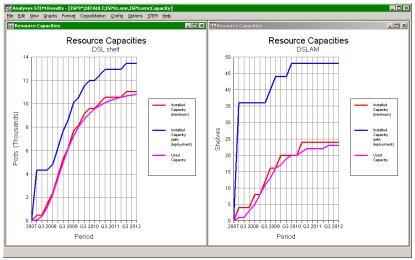
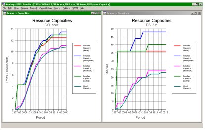
Used and installed equipment capacities
The deployment feature provides this awareness, and offers various alternative distribution
models for the spread of demand across those sites. The most generally useful is
the so-called Extended Monte Carlo distribution, which guarantees at least one unit
per site, and assumes an average of half a unit of slack capacity (240 ports) at
each site (even though the numbers will vary per site in practice). If you think
about it, this is a reasonable assumption in the absence of much more detailed data,
and captures a significant overhead cost (compared to the minimum installation)
which is sometimes neglected in hasty business plans.
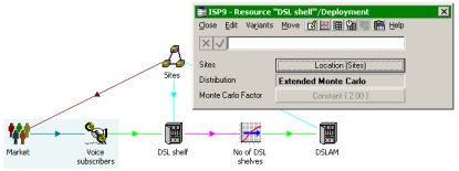
Extended Monte Carlo deployment
For both the DSL shelf and the DSLAM chassis itself, the evident effect is that
additional units must be installed long before 100% utilisation is reached. This
is because, across the sites in real life, there will be varying numbers of potential
households and different penetration rates, and some sites will reach 100% penetration
long before others do.
The remainder of this article demonstrates how you could progress to modelling the
sites individually if the detailed data were available, and how the installation
results compare.
Performing a manageable site-by-site calculation
Suppose we do have access to specific market size data on a per-site level, and
possibly even different penetration growth curves. Although we could run the model
over and over for each site in turn, this would not be very practical for a detailed
scenario or sensitivity analysis, nor would it give you results for the network
business as a whole.
This is why STEM provides a template replication feature which allows you to repeat
the same model structure many times within one model without having to manually
replicate any of the model structure. First you group the elements in question as
a template, and then you identify the inputs within that template which should vary
by site. STEM automatically creates a table with one row per input and one column
per site, and allows you to just type in the varying values without repeating the
entire calculation structure, ensuring consistency of calculation and results across
all sites.
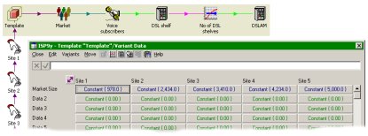
Template elements and variant data
Although manual replication is feasible with STEM’s intelligent copy-and-paste function,
this approach is labour intensive, subject to user error, and does not help much
if you want to add something to the calculation structure later. In contrast, template
replication allows you to identify template elements which will then be replicated
automatically whenever you re-run the model. This means that any new structure added
to the template will be automatically propagated across all sites.
Detailed and consistent results are generated for each individual site, as well
as for the network as whole. When you proceed to add scenarios or sensitivities,
you are guaranteed that these will impact equally on all sites. The further you
go with this sort of analysis, the harder it gets to keep everything consistent
in a spreadsheet, whereas STEM is purpose-built with this kind of process automation
in mind.
Template elements and variant data
Comparing the overall results with linear or normal demand distribution
The simplest use of this approach is to use a linear range of market sizes for the
various sites varying in the range 3000–7000 inclusive in steps of 500:
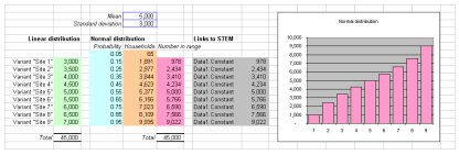
Linear and normal demand distributions
Or if we want to be more sophisticated, we can use an approximately normal distribution,
so that more of the sites are clustered towards the mean. This is an interesting
exercise in Excel (and in fact the numbers shown above are linked directly from
Excel into STEM), but as you will see from the charts below, it makes very little
difference to the overall results – no more than the impact of timing at the site
level.
Comparison with explicit linear and normal distributions
So the impact on the results of doing a very precise, site-level model is rather
slight compared to the significant difference between the ‘minimum’ results and
those factoring in the deployment, at least for the DSL shelf element. (The DSLAM
results deviate more because the utilisation is still critically low.)
STEM 7.1 consistently prompts you to consider equipment deployment, as it is listed
as a key feature in the top section of the Resource icon menu, and this is because
it can be such an important (and sometimes dominant) factor when dimensioning a
network.