 Subscriber churn, i.e. the turnover within
a subscriber base of new customers balanced by those leaving the network in a given period, is an inevitable
characteristic of competitive markets. STEM includes a Churn Proportion input for services which is propagated
through demand for resources and transformations to facilitate a straightforward and intrinsic calculation of
simple churn costs, such as a relocation expense for a re-assigned subscriber set-top box.
Subscriber churn, i.e. the turnover within
a subscriber base of new customers balanced by those leaving the network in a given period, is an inevitable
characteristic of competitive markets. STEM includes a Churn Proportion input for services which is propagated
through demand for resources and transformations to facilitate a straightforward and intrinsic calculation of
simple churn costs, such as a relocation expense for a re-assigned subscriber set-top box.
However, not all churn effects can be driven
by the churn proportion within the current period alone. This technical article describes approaches to modelling
two different churn situations: provision of new handsets for all new subscribers to a mobile network, and deployment
of final drops (from the kerb) to homes in a residential development.
Registered STEM users can
download the model files from this article.
Forecasting capex for handset provision
Mobile operators typically offer a handset
as part of a new subscription agreement. The so-called ‘handset subsidy’ refers to the fact that some or all of
the off-putting cost of a new handset is covered by the operator in return for a minimum term in the contract.
Consider a service with an annual churn rate,
c = 10%. In a given period, new handsets are required both for the explicit increase
in the number of contracted subscribers, x, but also for the hidden new subscribers replacing those who have left.
So in a period, n, the number of new customers
can be calculated as
(xn – xn–1) + xn · cn ·
lenn, where len is the length of the
period in years. (Only 2.5% will leave in a quarter of a year.)
Over time, the total demand for new handsets
will be the reported number of subscribers, plus the accumulation xi · ci · leni for i
= 0
to n. This is straightforward to model in
STEM:
- 10% is entered directly as the Churn Proportion input for a simple
Subscribers service.
- A multiplier transformation, Churners, takes the service demand in
connections as its input, and the multiplier is defined as
Subscribers.ChurnProp * periodLen (), using the built-in periodLen() function to capture
the length of each period in a time-series calculation.
- An expression transformation, Total churners, takes the output from
Churners as its input and defines its output as
prevThis (0) + Input1, using another built-in function designed specifically to facilitate
an accumulation without a circular reference.
- Another expression transformation, Total subscribers, takes the service
demand in connections as one input and Total churners as the second, and
defines its output in turn as Input1 + Input2.
- A requirement is defined from Total subscribers for a
Handset resource, which captures the initial capex per historical
subscriber.
Calculation of cumulative historical
subscribers vs. active subscribers.
Note: the Subscribers service and the
Total churners transformation could both drive the resource directly, and
achieve the sum implicitly, but we will need to reference the combined total again later, so the
Total subscribers transformation makes this cleaner.
Replacement
STEM automatically models
equipment replacement for a stable assignment of demand to a resource according to the resource’s Physical Lifetime
input. This case is more complicated because a proportion of handsets need not be renewed in future by the operator
because the relevant customers will have left (churned off) the network.
Suppose the desired replacement cycle is three years. First of all, the
Physical Lifetime of the original Handset resource is set to 15 years, long enough to avoid replacement
(within the model run) for all the historical Total subscribers.
Looking at the number of new handsets assigned
three years ago, yn
–3, a proportion,
ci of
their owners leave the network each year. So if
ci is
constant, the number needing to be replaced in year n can be calculated as yn–3 · (1 – c)3. (More generally, this could be expressed as yn–3 · (1 – cn–3) · (1 – cn–2) ·
(1 – cn–1) in an annual model, and you could
argue that the (1 – cn–3) term could be disregarded because of the minimum contract term.)
Again this is straightforward to model with
a time-lag transformation if churn is constant. If the incremental replacement demand in a period is always the
same constant proportion of the incremental total demand three years previously, it follows that the total replacement
demand over time is the same constant proportion of the original total demand three years previously:
- A time-lag transformation, Total subs
lag, takes the output from Total subscribers as its input, and defines
its output with a lag of three years.
- A multiplier transformation, Replacement
subs, takes the output from Total subs lag as its input, and the
multiplier is defined as (1 – Subscribers.ChurnProp) ^ 3.
- A requirement is defined from Replacement
subs for the same Handset resource, as it is likely that the same
handsets will be offered to all relevant subscribers who require a new or replacement handset in a given period.
(Choice of handset or change of supplier can be modelled separately, using this initial
Handset resource as a counter for the total number of handsets to be provided
over time.)
Active subscribers, cumulative historical subscribers and handset replacement
If the churn rate is not constant,
then the prevThis() function can be used again to have a parallel succession of transformations calculate the
gradually diminishing number of subscribers from one year to the next and requiring a replacement handset after
three years.
Modelling one-off infrastructure costs in a limited market
Consider a FTTH roll-out, where an
initial deployment of FTTC paves the way for final drops to individual homes in a residential development of
1000 homes. Because of competition with satellite and wireless providers, churn is just as much an issue here,
with the added twist that the final drop to a home really is a one-off cost: it need not be repeated if a new
subscriber moves into a house vacated by a former subscriber.
Each year, there will be a proportion of
new subscribers replacing leavers, so the number of final drops will gradually exceed the number of registered
subscribers. But this effect is clearly constrained by the size of the development, and so it impacts on the model
in two ways. First, the probability of a churned subscriber requiring a new drop is a function of the number of
cumulative drops to date, specifically (1000 – x – u
) / 1000, where u is the number of currently unused drops (i.e. the effective additional
churn), and x measures active subscribers as before.
In a given period, n, we could calculate the
increment to u as xn · cn · lenn ·
(1000 – xn–1 – un–1) / 1000, looking back one period to ensure that the formula avoids circularity.
Second, the number of unused drops at a given
point in time may exceed the difference between the number of active subscribers and total homes later if the
penetration is still growing. So we have to allow for the fact that an increase in the active subscriber base
may arise from a home which has previously been connected. In other words, the number of unused drops may decrease
as penetration increases. More precisely, we can calculate a decrement to u as (xn – xn–1) · u–1 / (1000 – x – 1),
again looking back one period for the probability to avoid a circularity.
These rules are readily captured in User Data
for a service, and then a one-off final drop resource can be driven by
x +
u:
- Market segment, Homes passed, defines the roll-out plan for FTTC.
- A service, FTTH, defines the penetration
into that addressable market.
- Select User Data from the icon menu for the service and, for each of the following
five items, select Rename Field from the Edit menu to customise these fields.
- Customers =
CustomerBase * Penetration.RefValue.
- Add drops = Customers * ChurnProp * periodLen () * prev (if (CustomerBase > 0,
(CustomerBase – Customers – “Unused drops”) / (CustomerBase – Customers), 0), 1).
- Sub drops =
(Customers – prev (Customers, 0)) * prev (if (CustomerBase > 0, “Unused drops” /
(CustomerBase – Customers), 0), 1).
- New unused drops =
min (“Add drops” – “Sub drops”, CustomerBase – Customers – prev (“Unused drops”, 0))
.
- Unused drops = prev (“Unused drops”, 0) + “New unused drops”.
- An expression transformation,
Homes with final drop, takes the service demand in connections as its input
(for cost allocation purposes), but defines its output directly as FTTH.Customers +
FTTH.“Unused drops”.
- A requirement is defined from Homes with final drop for a Final drop resource,
which captures the one-off capex per home.
Note the if
(CustomerBase > 0, …) checks in (5) and (6) and the rounding protection in (7).
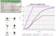
The following specimen results assume straight-line roll-out (to Y3) and penetration (to 60% in Y6) in order to
highlight the constrained churn effect.
Dynamic model of unused (and total) final drops
STEM Support offers mathematical insight and experience
These two examples are based on real-life STEM Support queries, where the main value-add from Implied Logic has been providing the mathematical insight to
rationalise the qualitative effects understood by the respective users and to transform them into quantitative
rules. Once a problem can be stated with mathematical equations, it is a matter only of experience to be able to
capture the equivalent logic in STEM and to fast-track to the results.
Registered STEM users can download the model files from this article.